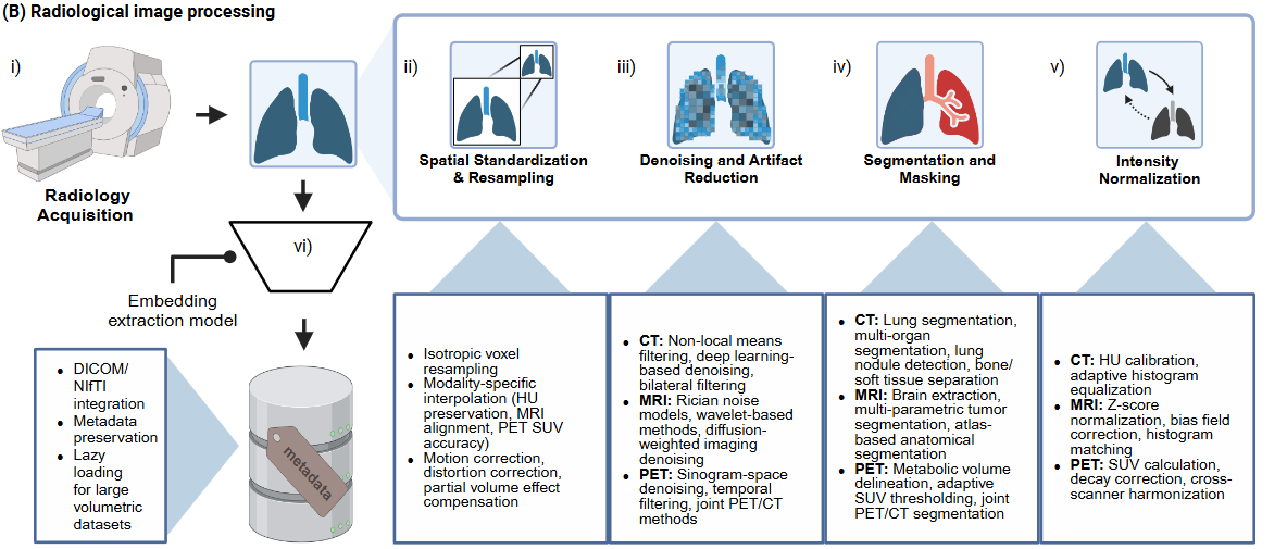
Overview
The radiology processing pipeline in HoneyBee handles Computed Tomography
(CT) imaging end-to-end: load DICOM series, inspect metadata, apply HU
windowing, preprocess (denoise, normalize, resample), segment lungs, and
generate embeddings with radiology foundation models. The
RadiologyProcessor class exposes every step as a standalone
method so you can compose custom pipelines or run the full chain with a
single call.
Key Features
- DICOM series loading with automatic slice ordering and metadata extraction
- Hounsfield Unit verification and 6 built-in window presets (lung, mediastinum, soft tissue, bone, abdomen, liver)
- Denoising (non-local means, bilateral) and intensity normalization (z-score, min-max, percentile)
- Isotropic resampling and bounding-box crop to ROI
- Lung segmentation via
lungmaskwith mask application - 7 radiology foundation model presets (RAD-DINO, MedSigLIP, REMEDIS, RadImageNet, TorchXRayVision)
- Slice-level and volume-level embedding aggregation (mean, max, median, std, concat)
- High-level
HoneyBee.process_radiology()one-call API
Quick Start
Install HoneyBee and download a sample CT DICOM series from HuggingFace:
import glob
import os

import numpy as np
import torch
from huggingface_hub import snapshot_download

from honeybee.processors.radiology import RadiologyProcessor

# Download CT DICOM samples from HuggingFace
data_dir = snapshot_download(
    repo_id="Lab-Rasool/honeybee-samples",
    repo_type="dataset",
    allow_patterns="CT/**",
)

# Find the DICOM series directory
dcm_files = glob.glob(os.path.join(data_dir, "CT", "**", "*.dcm"), recursive=True)
dicom_dir = os.path.dirname(dcm_files[0])
print(f"Found {len(dcm_files)} DICOM files in {dicom_dir}")

DEVICE = "cuda" if torch.cuda.is_available() else "cpu"
print(f"Device: {DEVICE}")Found 205 DICOM files in .../CT/1.3.6.1.4.1.14519.5.2.1...
Device: cudaDICOM Loading and Metadata
load_dicom() reads a directory of DICOM files, sorts slices by
position, and returns a 3-D NumPy volume plus an ImageMetadata
object with acquisition parameters.
processor = RadiologyProcessor(device=DEVICE)
image, metadata = processor.load_dicom(dicom_dir)

print(f"Volume shape:        {image.shape}")
print(f"Volume dtype:        {image.dtype}")
print(f"Value range:         [{image.min():.1f}, {image.max():.1f}]")
print(f"Modality:            {metadata.modality}")
print(f"Patient ID:          {metadata.patient_id}")
print(f"Pixel spacing:       {metadata.pixel_spacing}")
print(f"Slice thickness: {metadata.slice_thickness}")Volume shape: (104, 512, 512)
Volume dtype: int32
Value range: [-2048.0, 3072.0]
Modality: unknown
Patient ID:
Pixel spacing: (4.952378796116505, 0.976562, 0.976562)
Slice thickness: NoneAnatomical Landmarks and Volume Visualization
Named slice indices can be derived from the HU distribution to show each feature at its most relevant anatomy. Lung parenchyma (−900 to −400 HU) gives the lung extent; the heart is detected as a dip in lung area where it displaces parenchyma. This is not core HoneyBee functionality but useful for understanding the volume before processing.
from scipy.ndimage import binary_fill_holes

n_slices = image.shape[0]
h, w = image.shape[1], image.shape[2]

# Detect lung region via internal air cavities
lung_area = np.zeros(n_slices)
for i in range(n_slices):
    body = image[i] > -500
    internal_air = binary_fill_holes(body) & ~body
    lung_area[i] = (internal_air & (image[i] > -900) & (image[i] < -300)).sum()

# Lung-containing slices: > 2% of slice area
threshold = 0.02 * h * w
has_lung = np.where(lung_area > threshold)[0]

if len(has_lung) > 5:
    lung_start, lung_end = int(has_lung[0]), int(has_lung[-1])
    lung_extent = lung_end - lung_start

    # Orientation: diaphragm has steeper transition than apex
    quarter = max(3, lung_extent // 4)
    start_edge = lung_area[lung_start : lung_start + quarter]
    end_edge = lung_area[lung_end - quarter : lung_end + 1]
    start_steepness = np.max(np.abs(np.diff(start_edge))) if len(start_edge) > 1 else 0
    end_steepness = np.max(np.abs(np.diff(end_edge))) if len(end_edge) > 1 else 0
    apex_first = end_steepness > start_steepness

    if apex_first:
        SLICE_APEX, SLICE_BASES = lung_start, lung_end
    else:
        SLICE_APEX, SLICE_BASES = lung_end, lung_start

    # Heart: minimum lung area in the middle portion
    mid_lo = min(SLICE_APEX, SLICE_BASES) + lung_extent // 3
    mid_hi = max(SLICE_APEX, SLICE_BASES) - lung_extent // 4
    mid_range = np.arange(mid_lo, mid_hi + 1)
    SLICE_HEART = int(mid_range[np.argmin(lung_area[mid_range])])

    # Carina: 25% from apex toward bases
    direction = 1 if apex_first else -1
    SLICE_CARINA = SLICE_APEX + int(direction * lung_extent * 0.25)

print(f"Detected landmarks:  apex={SLICE_APEX}  carina={SLICE_CARINA}  "
f"heart={SLICE_HEART} bases={SLICE_BASES}")Detected landmarks: apex=6 carina=27 heart=55 bases=90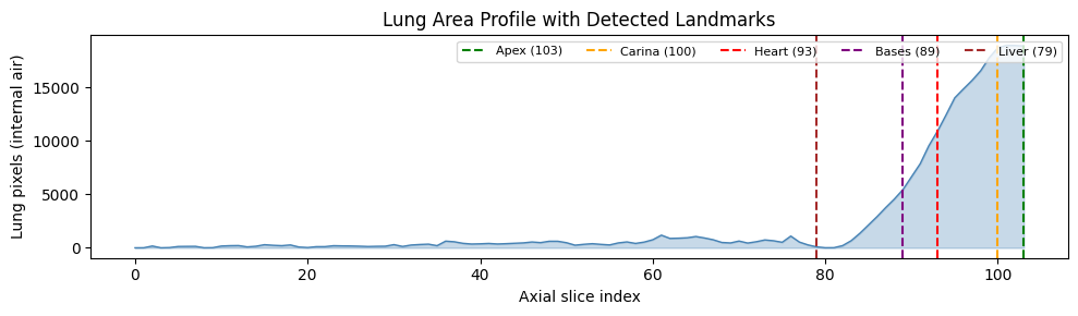
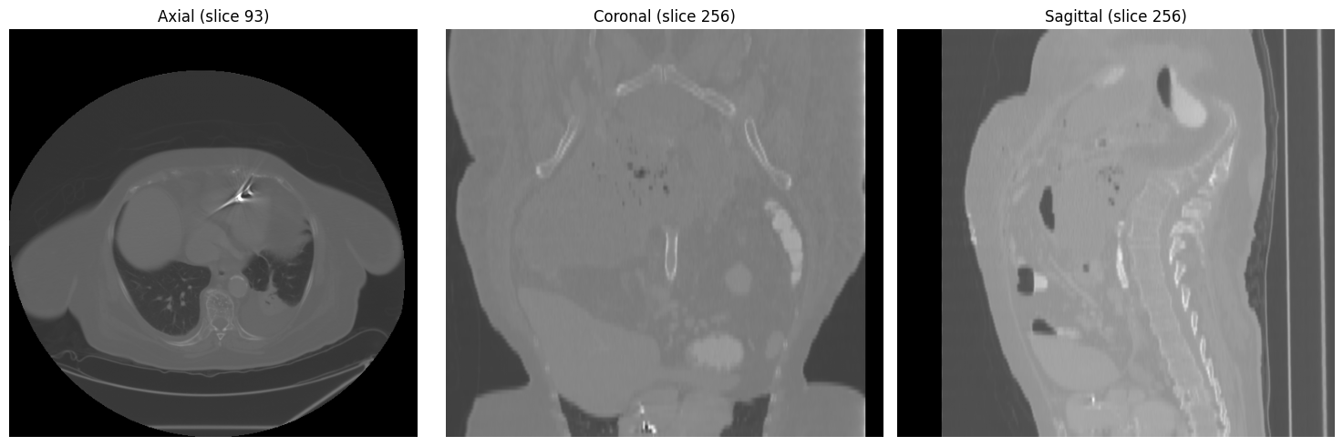
Three-view overview at mid-chest level (axial, coronal, sagittal):
HU Verification and Windowing
verify_hounsfield_units() checks whether the volume is in
proper HU scale and reports statistics. apply_window()
accepts named presets or custom (window, level) tuples.
hu_results = processor.verify_hounsfield_units(image, metadata)

print(f"Is HU:          {hu_results['is_hu']}")
print(f"Min value:      {hu_results['min_value']:.1f}")
print(f"Max value:      {hu_results['max_value']:.1f}")
print(f"Mean value:     {hu_results['mean_value']:.1f}")
print(f"Air present:    {hu_results['likely_air_present']}")
print(f"Bone present: {hu_results['likely_bone_present']}")Is HU: True
Min value: -2048.0
Max value: 3072.0
Mean value: -893.7
Air present: True
Bone present: TrueWindow Preset Comparison
Different window/level settings reveal different anatomical structures. Each preset is shown on the axial slice where that anatomy is most visible:
# Built-in presets: lung, mediastinum, soft_tissue, bone, abdomen, liver
preset_slices = {
    "lung":        SLICE_HEART,
    "mediastinum": SLICE_CARINA,
    "soft_tissue": SLICE_BASES,
    "bone":        SLICE_APEX,
    "abdomen":     SLICE_LIVER,
    "liver":       SLICE_LIVER,
}

fig, axes = plt.subplots(2, 3, figsize=(15, 10))
for ax, (preset, slice_idx) in zip(axes.flat, preset_slices.items()):
    windowed = processor.apply_window(image[slice_idx], window=preset)
    ax.imshow(windowed, cmap="gray")
    ax.set_title(f"{preset.replace('_', ' ').title()} (slice {slice_idx})")
    ax.axis("off")
Preprocessing Pipeline
The preprocessing pipeline provides denoising, intensity normalization, and
a combined preprocess() method that chains all steps based on modality.
Denoising Methods
Compare non-local means and bilateral denoising on a single slice, viewed through the soft-tissue window:
tissue_slice = image[SLICE_CARINA]
nlm_denoised = processor.denoise(tissue_slice, method="nlm")
bilateral_denoised = processor.denoise(tissue_slice, method="bilateral")

fig, axes = plt.subplots(1, 3, figsize=(15, 5))
for ax, img, title in zip(
    axes,
    [tissue_slice, nlm_denoised, bilateral_denoised],
    ["Original", "Non-Local Means", "Bilateral"],
):
    windowed = processor.apply_window(img, window="soft_tissue")
    ax.imshow(windowed, cmap="gray")
    ax.set_title(title)
    ax.axis("off")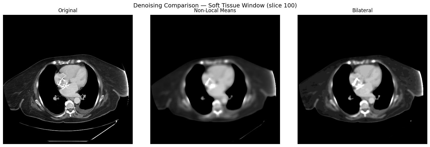
Intensity Normalization
Three normalization methods are available: z-score, min-max, and percentile.
methods = ["zscore", "minmax", "percentile"]
norm_slice = image[SLICE_HEART]

fig, axes = plt.subplots(1, 3, figsize=(15, 5))
for ax, method in zip(axes, methods):
    normalized = processor.normalize_intensity(norm_slice, method=method)
    ax.imshow(normalized, cmap="gray")
    ax.set_title(f"{method} — range [{normalized.min():.2f}, {normalized.max():.2f}]")
    ax.axis("off")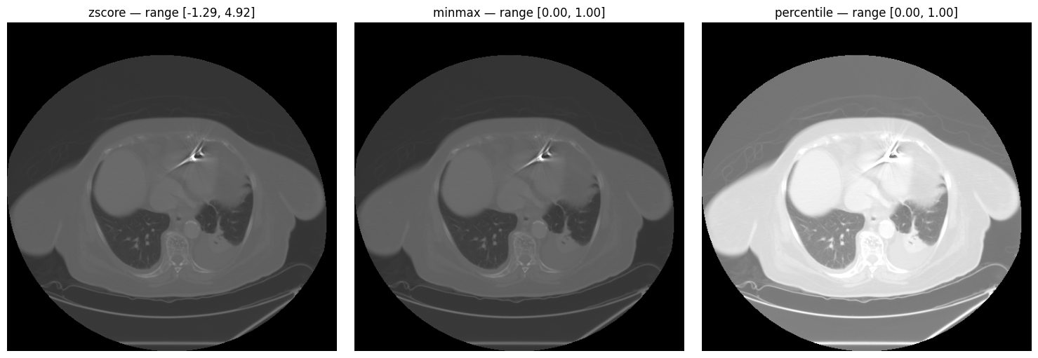
Full Pipeline
preprocess() chains denoising, windowing, and normalization in
a single call, configured by modality:
preprocessed = processor.preprocess(image, metadata)

print(f"Original shape:      {image.shape}")
print(f"Preprocessed shape:  {preprocessed.shape}")
print(f"Original range:      [{image.min():.1f}, {image.max():.1f}]")
print(f"Preprocessed range: [{preprocessed.min():.3f}, {preprocessed.max():.3f}]")Original shape: (104, 512, 512)
Preprocessed shape: (104, 512, 512)
Original range: [-2048.0, 3072.0]
Preprocessed range: [0.000, 1.000]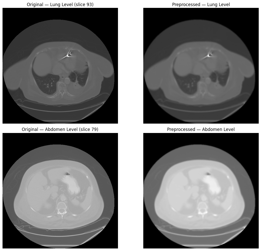
Spatial Operations
Standardize spatial resolution with isotropic resampling, and remove surrounding air with bounding-box cropping.
# Resample to isotropic 1mm spacing
resampled = processor.resample(image, metadata, new_spacing=(1.0, 1.0, 1.0))

print(f"Original shape:    {image.shape}")
print(f"Original spacing:  {metadata.pixel_spacing}")
print(f"Resampled shape:   {resampled.shape}")
print("Target spacing: (1.0, 1.0, 1.0)")Original shape: (104, 512, 512)
Original spacing: (4.952378796116505, 0.976562, 0.976562)
Resampled shape: (516, 500, 500)
Target spacing: (1.0, 1.0, 1.0)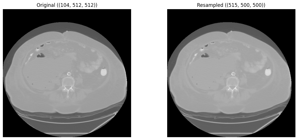
# Crop to body ROI (remove surrounding air)
body_mask = (image > -500).astype(np.uint8)
cropped = processor.crop_to_roi(image, body_mask)

print(f"Original shape:  {image.shape}")
print(f"Cropped shape: {cropped.shape}")Original shape: (104, 512, 512)
Cropped shape: (97, 340, 370)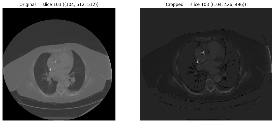
Lung Segmentation
segment_lungs() uses the
lungmask
library for automatic lung segmentation. The resulting binary mask can be
applied with apply_mask() to isolate lung parenchyma before
embedding generation.
lung_mask = processor.segment_lungs(image, spacing=metadata.pixel_spacing)

print(f"Mask shape:     {lung_mask.shape}")
print(f"Mask dtype:     {lung_mask.dtype}")
print(f"Lung voxels: {lung_mask.sum():,} ({lung_mask.mean():.2%} of volume)")Mask shape: (104, 512, 512)
Mask dtype: uint8
Lung voxels: 3,498,265 (12.83% of volume)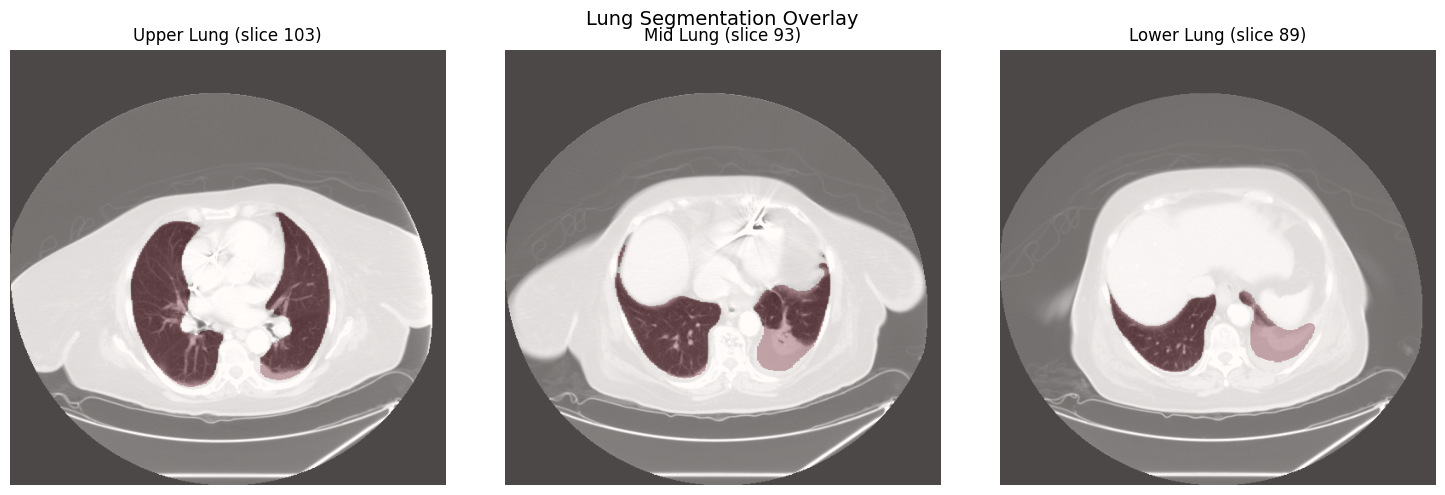
# Apply mask to isolate lung parenchyma
lung_only = processor.apply_mask(image, lung_mask)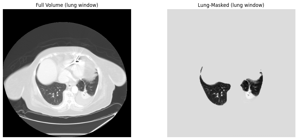
Embedding Generation
RadiologyProcessor wraps the model registry to generate
embeddings from CT volumes using radiology-specific foundation models.
Available Models
HoneyBee ships with 7 radiology model presets. Use list_models()
to see all available presets:
| Alias | Embedding Dim | Provider | Description |
|---|---|---|---|
rad-dino | 768 | huggingface | RAD-DINO radiology foundation model (Microsoft) |
medsiglip | 1152 | huggingface | MedSigLIP medical image-text model (Google) - 448x448 |
remedis | 2048 | onnx | REMEDIS CXR model (Google) - requires ONNX model_path |
radimagenet-resnet50 | 2048 | torch | RadImageNet ResNet50 pretrained model |
radimagenet-densenet121 | 1024 | torch | RadImageNet DenseNet121 pretrained model |
torchxrayvision-densenet | 1024 | torchxrayvision | TorchXRayVision DenseNet121 (all datasets, 224px) |
torchxrayvision-resnet | 2048 | torchxrayvision | TorchXRayVision ResNet50 (all datasets, 512px) |
Generate Embeddings
Initialize RadiologyProcessor with a model alias, then call
generate_embeddings(). For 3-D volumes, specify
mode="2d" and n_slices to sample and aggregate
across the volume:
processor_rd = RadiologyProcessor(model="rad-dino", device=DEVICE)
embeddings = processor_rd.generate_embeddings(image, mode="2d", n_slices=16)

print(f"Embeddings shape: {embeddings.shape}")
print(f"Embeddings norm: {np.linalg.norm(embeddings):.4f}")Embeddings shape: (768,)
Embeddings norm: 14.1231Slice-Level Aggregation
Generate per-slice embeddings and aggregate them into a volume-level representation using one of five methods:
# Generate per-slice embeddings
slice_indices = np.linspace(0, image.shape[0] - 1, 16, dtype=int)
slice_embeddings = np.stack(
    [processor_rd.generate_embeddings(image[i], mode="2d") for i in slice_indices]
)
print(f"Per-slice embeddings: {slice_embeddings.shape}")

# Available methods: mean, max, median, std, concat
for method in ["mean", "max", "median", "std", "concat"]:
    agg = processor_rd.aggregate_embeddings(slice_embeddings, method=method)
print(f" {method:>8s}: shape={agg.shape}, norm={np.linalg.norm(agg):.2f}")Per-slice embeddings: (16, 768)
mean: shape=(768,), norm=14.27
max: shape=(768,), norm=18.86
median: shape=(768,), norm=14.85
std: shape=(768,), norm=6.69
concat: shape=(1536,), norm=15.76HoneyBee High-Level API
process_radiology() runs the entire pipeline — DICOM
loading, preprocessing, and embedding generation — in a single call:
from honeybee import HoneyBee

honeybee = HoneyBee(config={"radiology": {"model": "rad-dino", "device": DEVICE}})
result = honeybee.process_radiology(
    dicom_path=dicom_dir, preprocess=True, generate_embeddings=True
)

print(f"Result keys:       {list(result.keys())}")
print(f"Image shape:       {result['image'].shape}")
print(f"Metadata modality: {result['metadata'].modality}")
if "embeddings" in result:
print(f"Embeddings shape: {result['embeddings'].shape}")Result keys: ['image', 'metadata', 'embeddings']
Image shape: (104, 512, 512)
Metadata modality: unknown
Embeddings shape: (768,)Complete Pipeline Example
Full end-to-end workflow from DICOM loading to volume-level embeddings:
import glob
import os

import numpy as np
import torch
from huggingface_hub import snapshot_download

from honeybee.processors.radiology import RadiologyProcessor

# 1. Download and locate DICOM series
data_dir = snapshot_download(
    repo_id="Lab-Rasool/honeybee-samples",
    repo_type="dataset",
    allow_patterns="CT/**",
)
dcm_files = glob.glob(os.path.join(data_dir, "CT", "**", "*.dcm"), recursive=True)
dicom_dir = os.path.dirname(dcm_files[0])
device = "cuda" if torch.cuda.is_available() else "cpu"

# 2. Load DICOM
processor = RadiologyProcessor(device=device)
image, metadata = processor.load_dicom(dicom_dir)

# 3. Verify HU scale
hu = processor.verify_hounsfield_units(image, metadata)
print(f"HU verified: {hu['is_hu']}")

# 4. Preprocess (denoise + normalize)
preprocessed = processor.preprocess(image, metadata)

# 5. Resample to isotropic spacing
resampled = processor.resample(preprocessed, metadata, new_spacing=(1.0, 1.0, 1.0))

# 6. Segment lungs and apply mask
lung_mask = processor.segment_lungs(image, spacing=metadata.pixel_spacing)
masked = processor.apply_mask(resampled, lung_mask)

# 7. Generate embeddings
processor_rd = RadiologyProcessor(model="rad-dino", device=device)
embeddings = processor_rd.generate_embeddings(masked, mode="2d", n_slices=16)

# 8. Aggregate to volume level
volume_embedding = processor_rd.aggregate_embeddings(
    embeddings.reshape(1, -1) if embeddings.ndim == 1
    else embeddings,
    method="mean",
)
print(f"Volume embedding: {volume_embedding.shape}")
Performance Considerations
When processing CT volumes, consider the following:
- GPU acceleration: Set
device="cuda"onRadiologyProcessorto run model inference on GPU - Slice sampling: Use
n_slicesingenerate_embeddings()to sample a representative subset rather than processing every slice - Preprocessing before embedding: Apply windowing and normalization to bring values into the expected model input range
- Lung masking: Segment and mask lungs before embedding to focus on relevant parenchyma and reduce noise from surrounding tissue
- Isotropic resampling: Resample to uniform spacing (e.g., 1mm isotropic) for consistent spatial representation across scans
- Memory management: CT volumes can be large; process slice-by-slice when memory is limited