Overview

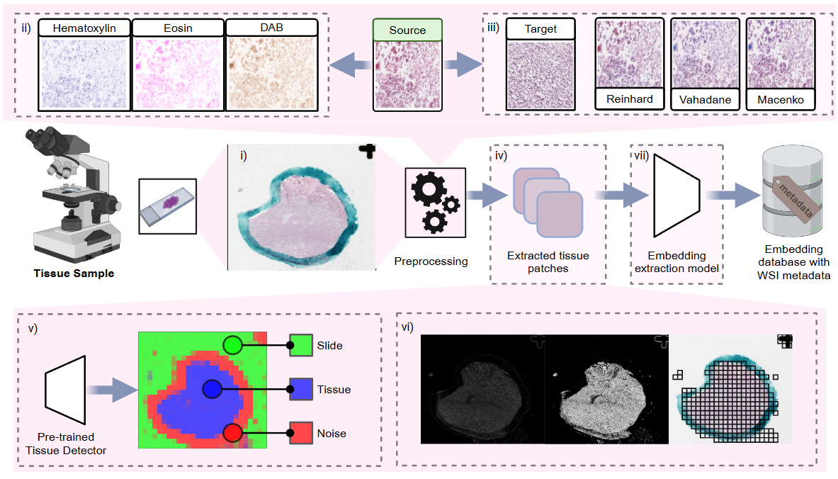
The pathology processing pipeline in HoneyBee handles Whole Slide Images (WSIs), which are high-resolution scans of tissue samples. These images present unique computational challenges due to their extreme size (often several gigabytes), multi-resolution pyramid structure, and vendor-specific file formats. HoneyBee uses a four-class modular design — Slide → PatchExtractor → Patches → PathologyProcessor — so each stage can be used independently or composed into end-to-end pipelines.

Key Features

• Support for multiple WSI formats (Aperio SVS, Philips TIFF, and more)
• Auto-detecting backend: CuCIM (GPU-accelerated) with OpenSlide fallback
• Deep-learning and classical tissue detection (Otsu, HSV, gradient)
• Stain normalization (Reinhard, Macenko, Vahadane) and H&E stain separation
• Grid-based patch extraction with tissue filtering and quality scoring
• 8 foundation model presets (UNI, UNI2, Virchow2, H-optimus, GigaPath, Phikon-v2, MedSigLIP, REMEDIS)
• Slide-level aggregation (mean, max, median, std, concat)
• Built-in visualizations: tissue masks, patch galleries, quality distributions, UMAP feature maps

Quick Start

Install HoneyBee with pathology dependencies and download a sample slide from HuggingFace:

import torch
from huggingface_hub import hf_hub_download

from honeybee.loaders.Slide.slide import Slide
from honeybee.processors import PathologyProcessor
from honeybee.processors.wsi import PatchExtractor

# Download a sample WSI from HuggingFace
SLIDE_PATH = hf_hub_download(
    repo_id="Lab-Rasool/honeybee-samples",
    filename="sample.svs",
    repo_type="dataset",
)

DEVICE = "cuda" if torch.cuda.is_available() else "cpu"

Slide Loading

The Slide class auto-detects the best available backend (CuCIM for GPU acceleration, OpenSlide as fallback) and provides a unified API for reading WSI files. Use slide.info to inspect metadata and slide.dimensions for the full-resolution size.

slide = Slide(SLIDE_PATH)

# Slide metadata (backend, dimensions, level count, magnification, etc.)
print(slide.info)

# Full-resolution dimensions (width, height)
print(slide.dimensions)  # e.g. (27965, 25146)

{
  "path": "sample.svs",
  "backend": "cucim",
  "dimensions": [27965, 25146],
  "level_count": 3,
  "level_dimensions": [[27965, 25146], [6991, 6286], [1747, 1571]],
  "level_downsamples": [1.0, 4.0, 16.0],
  "magnification": null,
  "mpp": 1.0,
  "vendor": null
}

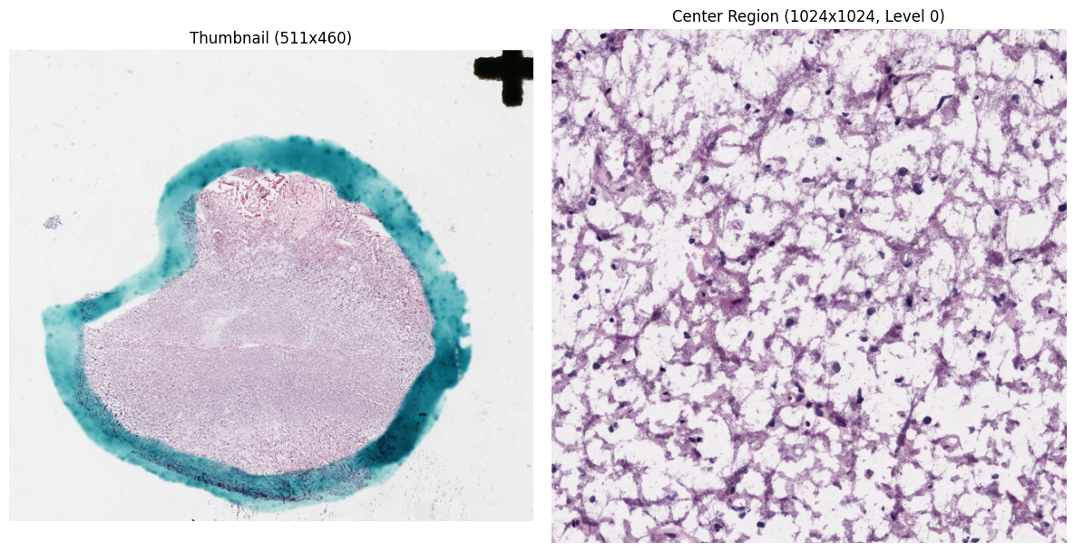
Thumbnails and Region Reading

get_thumbnail() returns a downsampled overview of the entire slide. read_region() reads pixels at a specific level-0 location and size, returning an RGB NumPy array.

# Downsampled overview
thumbnail = slide.get_thumbnail(size=(512, 512))

# Read a 1024x1024 region from the center of the slide
cx, cy = slide.dimensions[0] // 2, slide.dimensions[1] // 2
region = slide.read_region(
    location=(cx - 512, cy - 512),
    size=(1024, 1024),
    level=0,
)

Tissue Detection

HoneyBee provides both deep-learning and classical approaches for tissue detection. Results are stored on the slide object as slide.tissue_mask and slide.prediction_map.

Deep Learning Detection

Uses a pretrained DenseNet121 model for fine-grained tissue segmentation. The patch_size parameter controls tile resolution — smaller patches yield finer masks at the cost of more inference passes.

slide.detect_tissue(
    method="dl",
    device=DEVICE,
    patch_size=64,
    thumbnail_size=(4096, 4096),
)

print(f"Tissue mask: {slide.tissue_mask.shape}")
print(f"Tissue ratio: {slide.tissue_mask.mean():.2%}")
print(f"Prediction map: {slide.prediction_map.shape}")

# Visualize the detection result
slide.plot_tissue_detection()

Tissue mask: (3683, 4095), ratio: 29.48%
Prediction map: (24, 27, 3)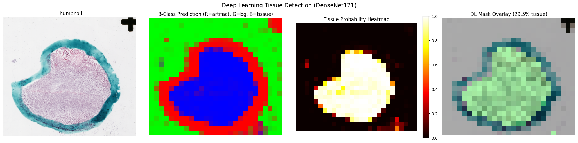

Classical Methods

Three classical approaches are available: Otsu thresholding ("otsu"), HSV color filtering ("hsv"), and their combination ("otsu_hsv").

# Otsu thresholding
slide.detect_tissue(method="otsu")

# HSV color filtering
slide.detect_tissue(method="hsv")

# Combined Otsu + HSV
slide.detect_tissue(method="otsu_hsv")

Method Comparison

Compare detection methods side-by-side to choose the best fit for your data:

slide.compare_tissue_methods(["dl", "otsu", "hsv", "otsu_hsv"])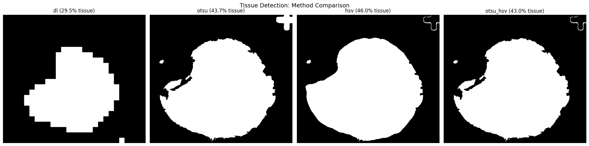

Patch Extraction

PatchExtractor performs grid-based extraction using the slide's tissue mask to filter out background tiles. Configure patch size, stride, and minimum tissue ratio to control density.

Grid Preview

Visualize the extraction grid over the tissue mask before committing to pixel reads:

extractor = PatchExtractor(
    patch_size=256,
    stride=256,
    min_tissue_ratio=0.5,
)

# Preview the grid overlay on the tissue mask
extractor.plot_grid_preview(slide)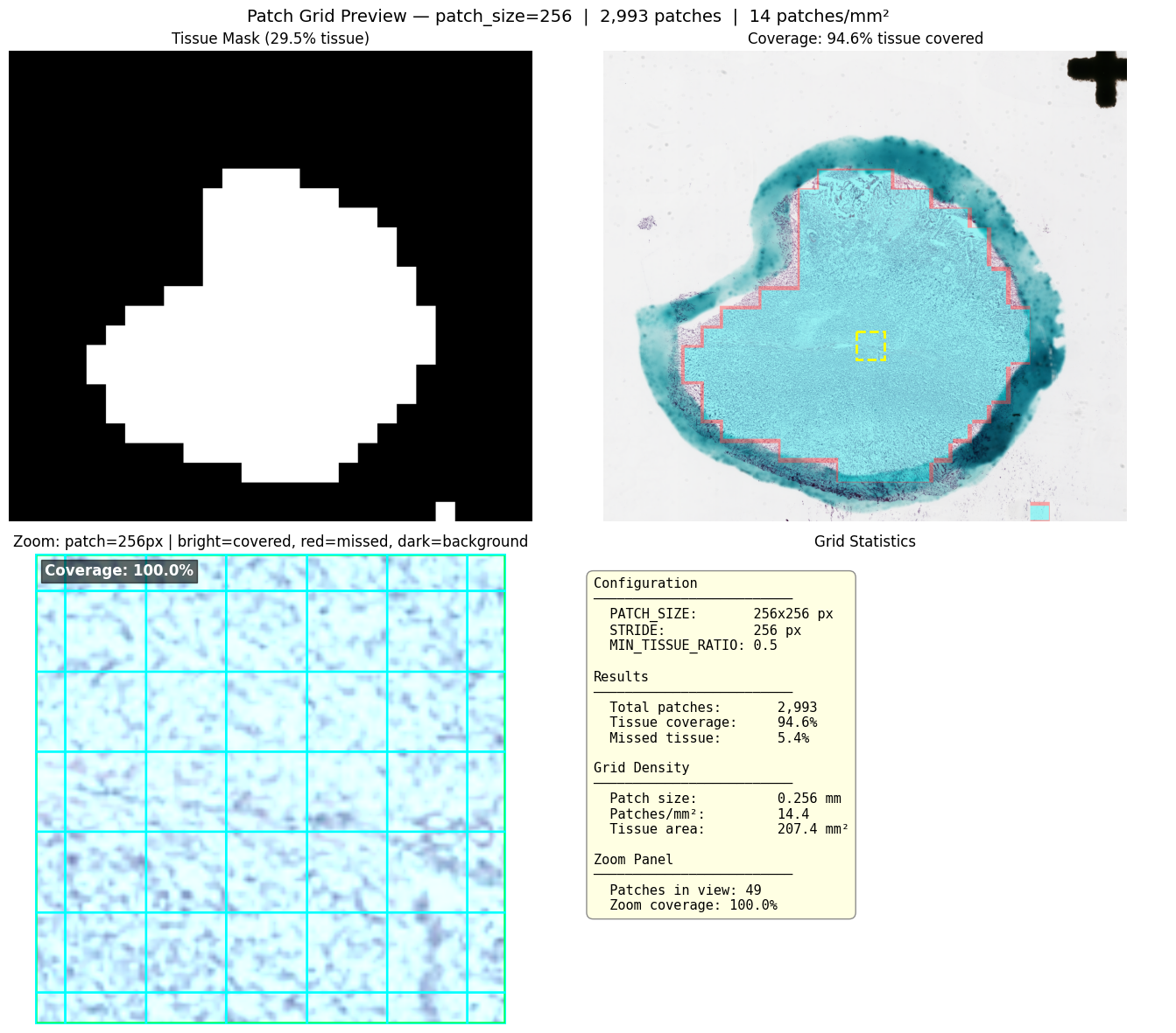

Extract and Inspect

extract() returns a Patches container holding image arrays and coordinates. Use built-in visualizations to inspect results.

patches = extractor.extract(slide)

print(f"Extracted {len(patches)} patches")
print(f"Images shape: {patches.images.shape}")
print(f"Coordinates shape: {patches.coordinates.shape}")

# Gallery of extracted patches
patches.plot_gallery(cols=8, max_patches=64)

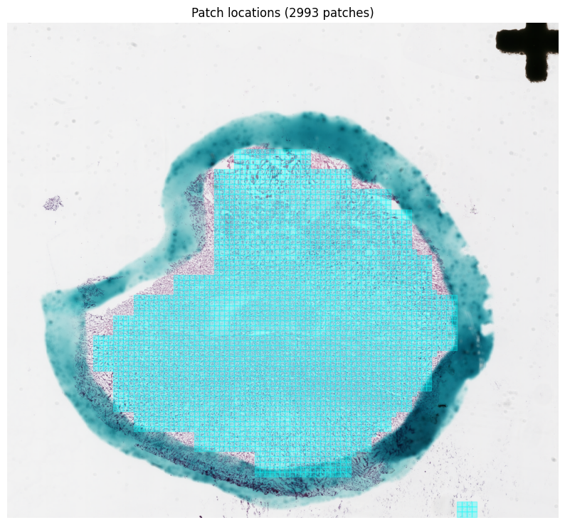
# Patch locations overlaid on the slide thumbnail
patches.plot_on_slide(slide)

Extracted 2993 patches
Images shape: (2993, 256, 256, 3)
Coordinates shape: (2993, 4)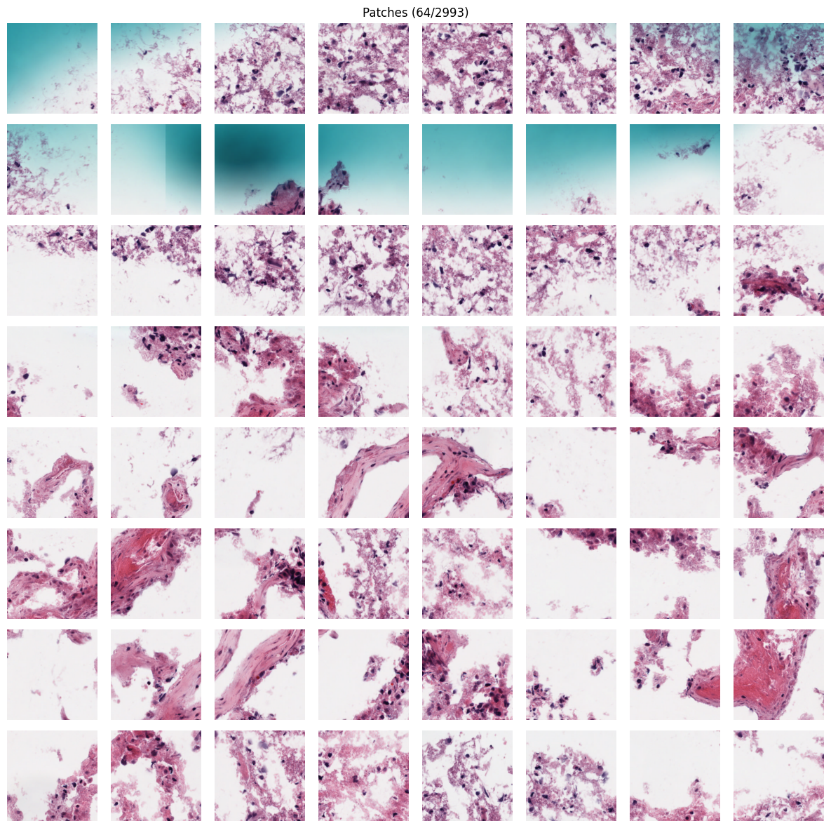

Quality Filtering

Quality scores combine tissue ratio, color variance, and edge content. Use plot_quality_distribution() to choose a threshold, then filter() to discard low-quality patches. The Patches container is immutable — filtering returns a new instance.

# Visualize quality score distribution with a threshold line
patches.plot_quality_distribution(threshold=0.7)

# Filter patches (returns a new Patches instance)
good_patches = patches.filter(min_quality=0.7)
print(f"Filtered: {len(patches)} -> {len(good_patches)} patches")

Filtered: 2993 -> 249 patches (min_quality=0.7)

Multi-Resolution Extraction

For large slides, run tissue detection at low magnification to build a coarse spatial grid, then pass it to a high-resolution extractor via the tissue_coordinates parameter. This avoids re-running detection at full resolution.

# Low-res tissue grid: small patches at coarse magnification
lowres_extractor = PatchExtractor(
    patch_size=16, stride=16, magnification=5.0, min_tissue_ratio=0.3
)
tissue_grid = lowres_extractor.get_coordinates(slide)
print(f"Low-res tissue grid: {len(tissue_grid)} tiles")

# High-res extraction using the tissue grid as a spatial filter
hires_extractor = PatchExtractor(
    patch_size=256, stride=256, magnification=20.0, min_tissue_ratio=0.5
)
hires_patches = hires_extractor.extract(slide, tissue_coordinates=tissue_grid)
print(f"High-res patches: {len(hires_patches)}")

Low-res tissue grid: 809280 tiles (16px @ ~5x)
High-res patches: 3188 (256px @ ~20x)
Tissue filter: tissue_coordinates
Tissue coordinates used: 809280

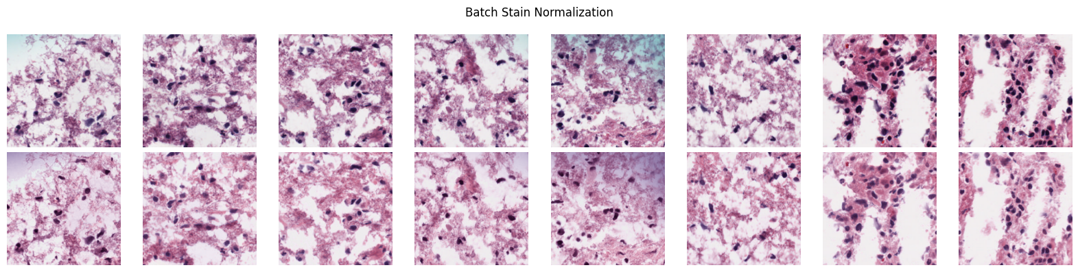
Stain Normalization

Stain normalization reduces color variability across slides from different scanners and labs. Three methods are available: Reinhard, Macenko, and Vahadane. All stain operations on Patches are immutable and return new instances.

# Compare all normalization methods side-by-side on a single patch
good_patches.plot_normalization_comparison()

# Apply Macenko normalization (returns a new Patches instance)
normalized = good_patches.normalize(method="macenko")

# Before/after visualization
good_patches.plot_normalization_before_after(normalized)

Normalized 249 patches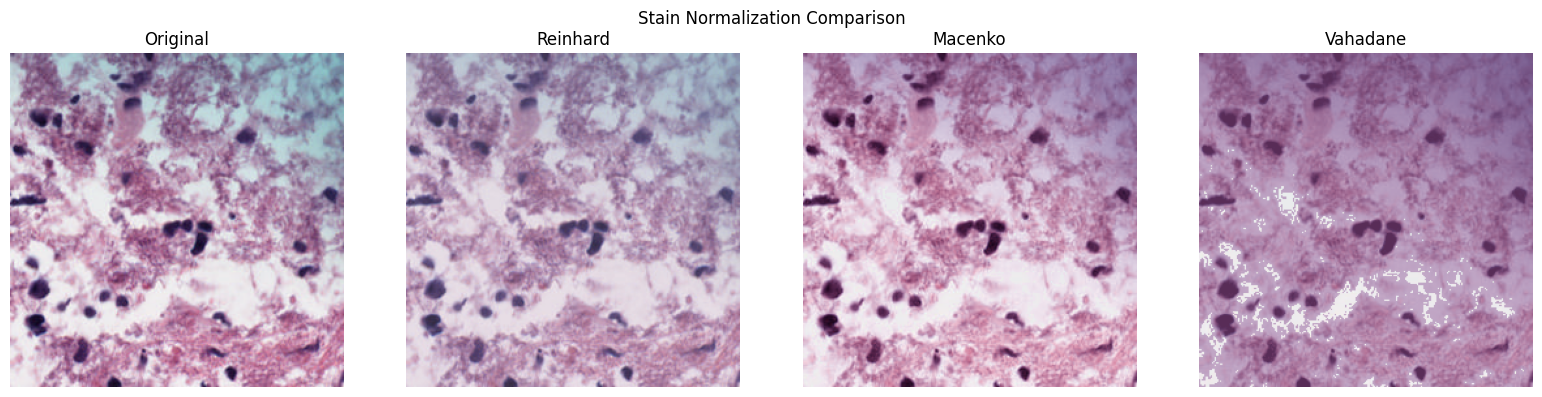

H&E Stain Separation

Deconvolve patches into hematoxylin, eosin, and background channels using color deconvolution:

patches.plot_stain_separation()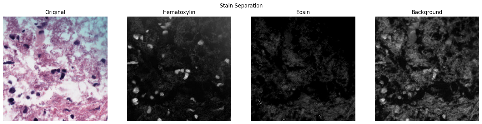

Embedding Generation

PathologyProcessor wraps the model registry to generate patch-level embeddings from any supported foundation model. Pass a Patches object directly to generate_embeddings().

Available Models

HoneyBee ships with 8 preset foundation models. Use list_models() to see all available presets, or pass any HuggingFace / timm model ID with an explicit provider.

from honeybee.models.registry import list_models

# List all registered model presets
for m in list_models():
    print(f"  {m['alias']:>12s}  dim={m['embedding_dim']:>4d}  provider={m['provider']}")

      gigapath  dim=1536  provider=timm
     h-optimus  dim=1536  provider=timm
     medsiglip  dim=1152  provider=huggingface
     phikon-v2  dim=1024  provider=huggingface
       remedis  dim=2048  provider=onnx
           uni  dim=1024  provider=timm
          uni2  dim=1536  provider=timm
      virchow2  dim=2560  provider=timm

Generate Embeddings

Initialize PathologyProcessor with a model alias, then call generate_embeddings() with a Patches object:

processor = PathologyProcessor(model="uni2")

# Inspect model configuration
info = processor.get_model_info()
print(f"Model: {info['alias']}, dim: {info['embedding_dim']}")

# Generate patch-level embeddings
embeddings = processor.generate_embeddings(
    patches,
    batch_size=32,
    progress=True,
)
print(f"Embeddings shape: {embeddings.shape}")  # (num_patches, embedding_dim)

Model: uni2, dim: 1536
Embeddings shape: (2993, 1536)

Slide-Level Aggregation

Aggregate patch-level embeddings into a single slide-level representation using one of five methods:

# Available methods: mean, max, median, std, concat
for method in ["mean", "max", "median", "std", "concat"]:
    agg = processor.aggregate_embeddings(embeddings, method=method)
    print(f"  {method:>8s}: shape={agg.shape}")

      mean: shape=(1536,)
       max: shape=(1536,)
    median: shape=(1536,)
       std: shape=(1536,)
    concat: shape=(3072,)

UMAP Feature Maps

Project high-dimensional embeddings to 3D with UMAP, map each dimension to an RGB channel, and overlay on the slide thumbnail. Similar tissue regions receive similar colors.

processor.plot_feature_map(patches, embeddings, slide)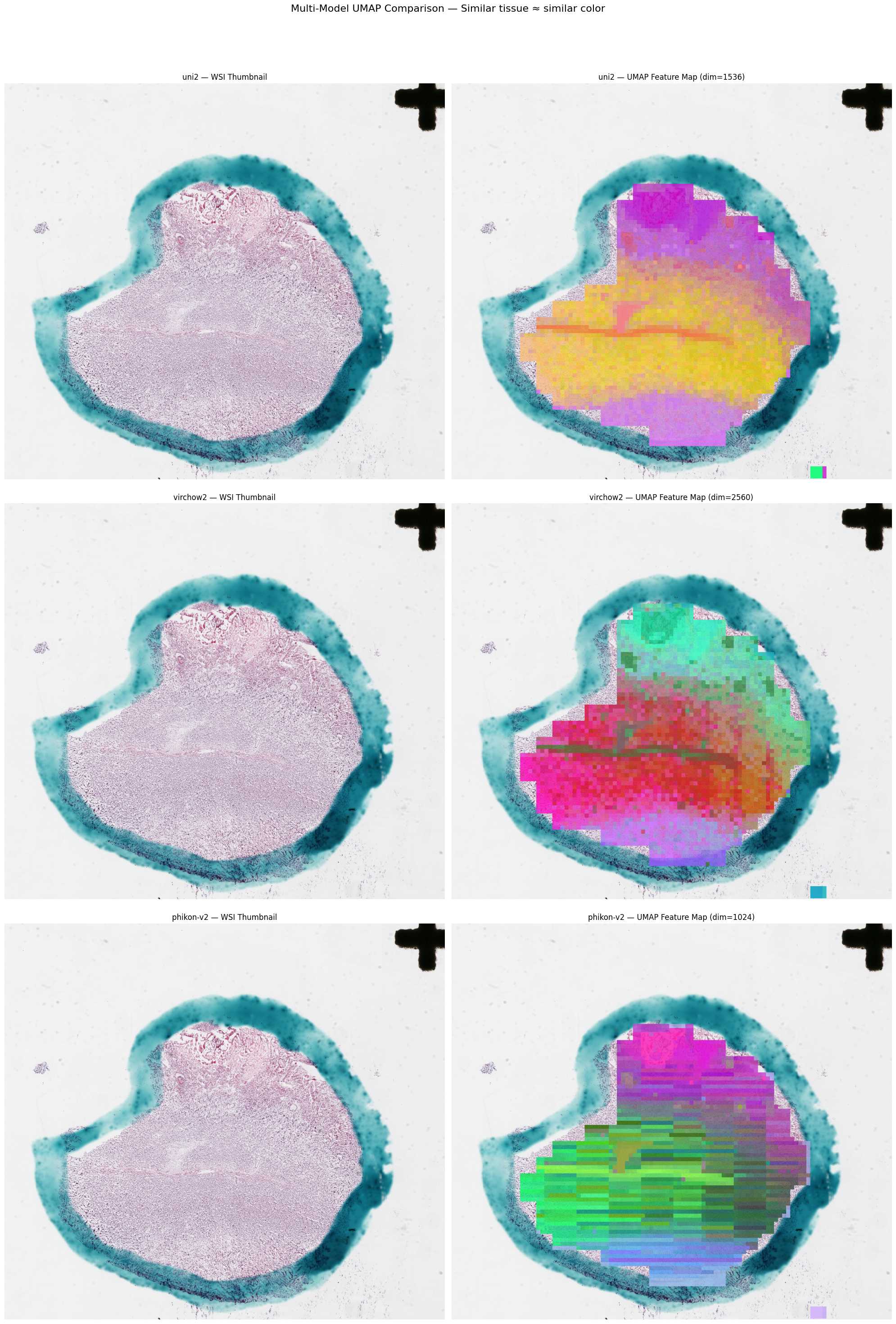

Complete Pipeline Example

Full end-to-end workflow from WSI loading to slide-level embeddings:

import torch
from huggingface_hub import hf_hub_download

from honeybee.loaders.Slide.slide import Slide
from honeybee.processors import PathologyProcessor
from honeybee.processors.wsi import PatchExtractor

# 1. Load slide
slide_path = hf_hub_download(
    repo_id="Lab-Rasool/honeybee-samples",
    filename="sample.svs",
    repo_type="dataset",
)
slide = Slide(slide_path)

# 2. Detect tissue
device = "cuda" if torch.cuda.is_available() else "cpu"
slide.detect_tissue(method="dl", device=device, patch_size=64)

# 3. Extract patches
extractor = PatchExtractor(patch_size=256, stride=256, min_tissue_ratio=0.5)
patches = extractor.extract(slide)

# 4. Quality filtering
good_patches = patches.filter(min_quality=0.7)

# 5. Stain normalization
normalized = good_patches.normalize(method="macenko")

# 6. Generate embeddings
processor = PathologyProcessor(model="uni2")
embeddings = processor.generate_embeddings(normalized, batch_size=32, progress=True)

# 7. Slide-level aggregation
slide_embedding = processor.aggregate_embeddings(embeddings, method="mean")
print(f"Slide embedding: {slide_embedding.shape}")

# 8. Visualize
processor.plot_feature_map(normalized, embeddings, slide)

Performance Considerations

When processing large WSIs, consider the following:

• CuCIM backend: Automatically preferred when available; provides GPU-accelerated slide reading
• Thumbnail-resolution detection: Run tissue detection on downsampled thumbnails to save time on initial segmentation
• Multi-resolution extraction: Build a coarse tissue grid at low magnification, then pass it to a high-resolution extractor via tissue_coordinates
• Batch sizes: Tune batch_size in generate_embeddings() to balance GPU memory and throughput
• Quality filtering before embedding: Filter out low-quality patches before the expensive embedding step to avoid wasted compute
• Immutable Patches: filter(), normalize(), and slicing return new Patches instances — the original is never modified